Creating a SCD Type 2 mapping using the Informatica PowerCenter Mapping Wizard

The Mapping Wizard available in the Informatica PowerCenter Designer client provides pre-designed mapping templates to create mappings based on specific requirements like SCD Types 1, 2 & 3.

The example below explains the creation of an SCD Type 2 mapping using the Mapping Wizard. The source table is EMPLOYEES that contains employee information like Employee ID, Name, Role, Department ID, Location, Employment Status and the Date of joining.

The EMPLOYEES table is shown below.

EMPLOYEES
EMP_ID	EMP_NAME	EMP_ROLE	DEPT_ID	LOCATION	EMPL_STATUS	JOIN_DT
1321	Shaun Mathews	Clerk	209	Atlanta	Active	13-Apr-08
1487	Shane Smith	Supervisor	110	Atlanta	Active	4-Aug-08
1678	Katie Wells	Manager	198	Atlanta	Active	20-Aug-08

The field EMP_ID is the primary key for the EMPLOYEES table. The fields on which history needs to be maintained are EMP_ROLE, DEPT_ID, LOCATION and EMPL_STATUS.

Import the source definition EMPLOYEES using the Source Analyzer workspace. Go to Sources > Import from Database.

This opens the Import Tables window. Assuming that a system DSN is already created for this connection, specify all the necessary details and click Connect.

Select the EMPLOYEES table to import and click OK to continue.

The EMPLOYEES source definition is created and appears in the workspace. Click Save to save the source definition in the repository.

The source table EMPLOYEES contains only current data and doesn't have any historical data. This mapping would be run daily to capture the historical data in the EMPLOYEES_SCD2 target table. The Effective Date logic would be used for SCD Type 2 mapping.

Click on the Mapping Designer tab.

Go to Mappings >  Wizards > Slowly Changing Dimensions.

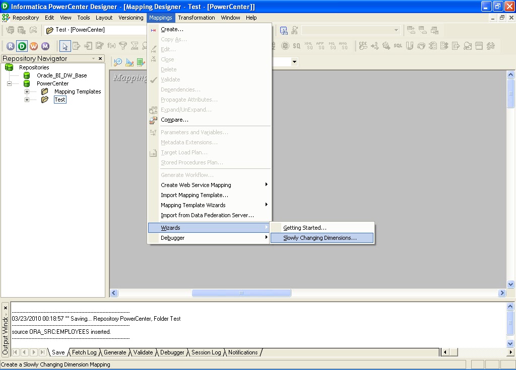
Provide a suitable mapping name as shown and select the Type 2 Dimension radio button. Click Next to continue.

Select the correct Source definition from the Select Source Table drop-down list and type the New Target Table name as EMPLOYEES_SCD2 as shown. Click Next to continue.

This opens the Target Field Selection window as shown.

Add the EMP_ID field as Logical Key Fields as shown as it is the primary key in the EMPLOYEES source table and it will be a part of the Lookup Transformation condition to check if the employee record is present in the EMPLOYEES_SCD2 target table.

Add the remaining fields on which history needs to be maintained as Fields to compare for changes as shown.

Click Next. Select Mark the dimension records with their effective date range as the versioning method to maintain history.

This adds two more fields PM_BEGIN_DATE and PM_END_DATE to the EMPLOYEES_SCD2 target table, which helps identify the effective start date and the end date respectively for each employee's record and if any of the fields on which history needs to be tracked undergo a change in the source table, a new record for that employee will be created with new effective start date and end date will be null. The PM_END_DATE value will be null for all current version of the records in the EMPLOYEES_SCD2 table. The date logic is indeed useful in scenarios wherein the source system doesn't have an effective date or last updated date field and it is binding on the ETL system to provide such a function. However, the definiteness of the effective start and end date being loaded into the history table will also depend on the frequency at which the SCD Type 2 mapping is run.

Click Finish.

The SCD Type 2 mapping is generated.

Save the mapping in the repository by pressing Ctrl+S. Check the Output Window below which displays messages stating that the mapping is valid with no parsing errors.

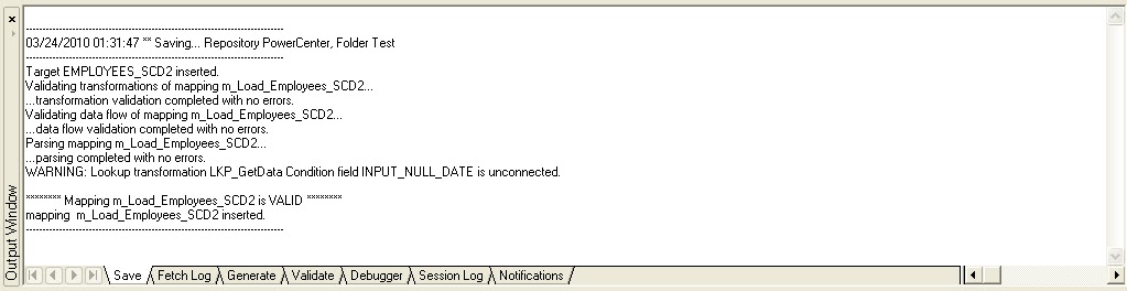
The new target definition EMPLOYEES_SCD2 is created in Informatica Designer, but not in the database.

Drag the target definition EMPLOYEES_SCD2 from the Repository Navigator into the Target Designer workspace.

Go to Targets > Generate/Execute SQL.

This opens the Database Object Generation window. Mention the path and filename for the DDL file to be created. Select the Create table radio button under the Generation options. Select the Create index radio button.

Click Generate and execute.

This opens the Connect to an ODBC Data Source window. Mention the necessary database details where the target table should be created and click Connect.

Check the Output Window to verify if the script has been successfully generated and executed in the database.

Click Close to close the Database Object Generation window.

The iconic view of the mapping is shown below.

A brief description of the transformations used in the mapping is given below.

1.    LKP_GetData: This is a lookup on the target table EMPLOYEES_SCD2 and will compare the incoming data from the EMPLOYEES source table based on the key field EMP_ID with that of the target table, EMPLOYEES_SCD2. All the currently active records in the EMPLOYEES_SCD2 table will have a null PM_END_DATE. Hence, only these records should be compared for changes with the incoming data and therefore, an unconnected input port INPUT_NULL_DATE is also matched with the PM_END_DATE field of the lookup table as part of the Condition. The condition used in the lookup transformation LKP_GetData is shown below.

2.    EXP_DetectChanges: This expression transformation will generate two flags - ChangedFlag and NewFlag. The ChangedFlag will check if the employee information in the EMPLOYEES_SCD2 target table has undergone a change in the source EMPLOYEES table. The NewFlag will check for the occurrence of new employee records in the source EMPLOYEES table.

3.    SEQ_GenerateKeys: This sequence generator generates unique keys for the PM_PRIMARYKEY field in the EMPLOYEES_SCD2 table for both new records and records that have undergone change in the fields on which history is maintained in the EMPLOYEES source table, which will be inserted as a new record in the target table.

4.    EXP_KeyProcessing_InsertNew & EXP_KeyProcessing_InsertChanged: The expression transformations EXP_KeyProcessing_InsertNew & EXP_KeyProcessing_InsertChanged generate the effective start date PM_BEGIN_DATE for the new records and the changed records that are inserted into the EMPLOYEES_SCD2 target table respectively.

5.    FIL_InsertNewRecord, FIL_InsertChangedRecord & FIL_UpdateChangedRecord: The filter transformation FIL_InsertNewRecord passes the new rows if the NewFlag is TRUE while the filter transformations - FIL_InsertChangedRecord & FIL_UpdateChangedRecord passes the changed rows if the ChangedFlag is TRUE.

6.    UPD_ForceInserts, UPD_ChangedInserts & UPD_ChangedUpdate: The update strategy transformations UPD_ForceInserts & UPD_ChangedInserts are used to manage inserts for new rows and changed rows respectively while the UPD_ChangedUpdate is used to update the old version rows based on the PM_PRIMARYKEY field.

7.    EXP_CalcToDate: This expression transformation generates the effective end date PM_END_DATE for the old version of an employee’s record in the EMPLOYEES_SCD2 target table.

The only optimization needed in the mapping is replacing the three filter transformations with a router transformation.

Create a valid session and workflow for this mapping.

Start the Workflow Manager client tool and click on the Task Developer tab. Go to Tasks > Create to create a new task.

This opens the Create Task window. Select the Session task from the drop-down and enter a name for this task as shown below.

Click Create to continue. Select the mapping created in the previous steps to associate with this session.

Click OK to continue. Click Done in the Create Task window.

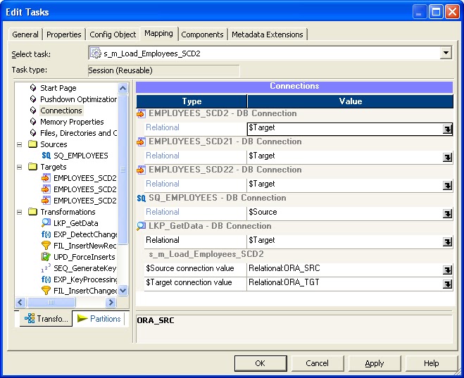
A new task is created in the Task Developer workspace as shown above. Double click on the session to edit it. Click on the Mapping tab and select the Connections option on the left and apply the correct relational connections as shown below.

Click OK to continue. Right click on the session task and click Validate to validate the session as shown below.

A notification is generated in the Output Window as shown below stating that the session is valid.

Press Ctrl+S to save the session task.

Click on the Workflow Designer tab. Go to Workflows > Create to create a new workflow.

This opens the Create Workflow window. Provide the workflow name as shown below.

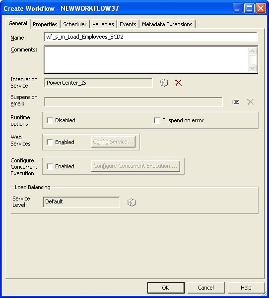
Click OK. Drag the session created in the previous steps from the Repository Navigator into the Workflow Designer workspace. Go to Tasks > Link Task.

Link the Start task to the session task as shown below.

Click Ctrl+S to validate and save the workflow.

Assuming the workflow ran for the first time on the 24th March, 2010, the data loaded in the target table is shown below. Click on the image to see the enlarged view.

Observing the data in the target table, it is evident that since all these records are the current version, the PM_END_DATE for all these records are null.

Assuming that the role of Shane Smith changes to Manager and the department ID of Katie Wells changes to 151 in the source system and a new employee, Jim Mason joins the organization on the 25th March, 2010, the EMPLOYEES table is shown below.

EMPLOYEES
EMP_ID	EMP_NAME	EMP_ROLE	DEPT_ID	LOCATION	EMPL_STATUS	JOIN_DT
1321	Shaun Mathews	Clerk	209	Atlanta	Active	13-Apr-08
1487	Shane Smith	Manager	110	Atlanta	Active	4-Aug-08
1678	Katie Wells	Manager	151	Atlanta	Active	20-Aug-08
2050	Jim Mason	Clerk	171	Chicago	Active	25-Mar-10

After the workflow runs on the 25th March, 2010, the data loaded in the target table is shown below. Click on the image to see the enlarged view.

The old version of records for Shane Smith and Katie Wells have been updated with a PM_END_DATE of 25-Mar-10 and two new versions of records having PM_PRIMARYKEY values 5 and 6 and a null value for PM_END_DATE get inserted into the target table. The new record for Jim Mason also gets inserted into the target table with a null value for PM_END_DATE, indicating it is the current version of the record in the target table.

Reporting the difference rows between two sources using Informatica

The purpose of the mappings discussed below are to report the difference rows between two sources in different scenarios.

Scenario 1: When there are difference rows in one of the sources and both the sources are either flat files or a flat file and a relational table.
To illustrate this scenario, the two sources considered are two comma separated flat files - EMPLOYEE_FILE_1.txt and EMPLOYEE_FILE_2.txt. The EMPLOYEE_FILE_2.txt has some extra records that need to be reported or loaded into the target which is a relational table having the same definition as the sources. The difference rows between the two flat files are highlighted in red as shown below.

Import the two flat file definitions using the Source Analyzer in Informatica PowerCenter Designer client tool as shown below.

Create a new mapping in the Mapping Designer and drag the two source definitions into the workspace.
Now, to identify the extra records from EMPLOYEE_FILE_2, a Joiner transformation followed by a Filter transformation is used.

The illustration discussed below uses an unsorted Joiner Transformation and since both the sources are having few records, any one of the sources can be treated as the "Master" source. Here the EMPLOYEE_FILE_1 source is designated as the "Master" source. In practice, however, to improve performance for an unsorted joiner transformation, the source with fewer rows is treated as the "Master" source while for a sorted joiner transformation, the source with fewer duplicate key values is assigned as the "Master" source.

First drag all the ports from the source qualifier SQ_EMPLOYEE_FILE_2 into the joiner transformation. Notice the ports created in the joiner transformation are designated as the "Detail" source by default. Drag only the EMP_ID port from SQ_EMPLOYEE_FILE_1 into the joiner transformation as shown below.

Double-click the joiner transformation to open up the Edit view of the transformation. Click on the Condition tab and specify the condition shown below.

Since, we need to pass all the rows from the EMPLOYEE_FILE_2, the Join Type used is "Master Outer Join" in the Properties tab as shown below. This will ensure that all the rows from the "Detail" source and only the matching rows from the "Master" source will pass from the joiner transformation.

The Join types supported in the joiner transformation are described below.

The rows passed by the joiner transformation are shown below. For the missing rows in the "Master" source, the EMP_ID1 value is NULL.

Now, a filter transformation can be used ahead to pass only the records having EMP_ID1 as NULL since these rows correspond to the difference rows from EMPLOYEE_FILE_2 source. Pass all the rows from the joiner transformation into the filter transformation and add the Filter condition shown below in the Properties tab of the filter transformation.

The records passed by the filter transformation are shown below.

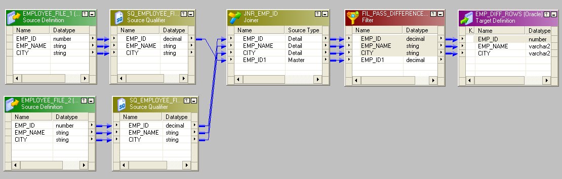
Link the EMP_ID, EMP_NAME and CITY ports to the target definition. The complete mapping is shown below.

Create a session task and a workflow. After running the workflow, the difference rows loaded into the target relational table are shown below.

Scenario 2: When there are difference rows in both the sources and both the sources are either flat files or a flat file and a relational table.
For this illustration, we consider both the sources are flat files. The difference rows in both the flat files are highlighted in red. The target relational table has an additional column SOURCE_NAME added, which indicates the source name where the difference row is present.

The EMPLOYEE_FILE_1 is treated as the "Master" source again for the unsorted joiner transformation. All the ports from the source qualifier SQ_EMPLOYEE_FILE_1 are passed to the joiner transformation as shown below because the difference records are present in both the sources.

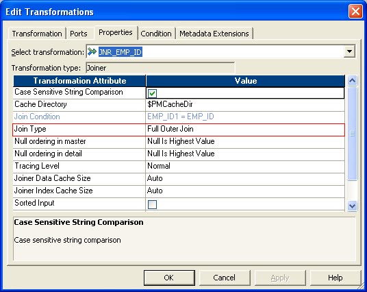
The join condition for the joiner transformation is the same as the first scenario, but for this case, the Join Type is Full Outer Join as shown below.

The rows passed by the joiner transformation are shown below. For the missing rows in the "Master" source, the EMP_ID1, EMP_NAME1 and CITY1 values are NULL, while for the missing rows in the "Detail" source, the EMP_ID, EMP_NAME and CITY values are NULL.

The filter transformation shown below should only pass the rows having NULL values in EMP_ID or EMP_ID1 ports as these correspond to the difference rows in the EMPLOYEE_FILE_2 and EMPLOYEE_FILE_1 flat files respectively.

The filter condition used in the filter transformation is shown below.

The filter transformation passes the following rows.

Now, add an expression transformation after the filter transformation. Pass all the ports from the filter transformation to the expression transformation. The expression transformation should have the following ports in the order shown below.

The logic for the output port EMP_ID_OUT is that if the EMP_ID value from EMPLOYEE_FILE_2 source is NULL, pass the EMP_ID1 value from the EMPLOYEE_FILE_1 source, else return the EMP_ID value from EMPLOYEE_FILE_2 source. This logic works because for any row passed from the filter transformation, either the row from the "Master" source will have NULL values or the row from the "Detail" source will have NULL values. A similar logic is applied for the EMP_NAME_OUT and CITY_OUT output ports.

Another output port SOURCE_NAME_OUT is used to determine the source of the difference row. The expression used for this port is shown below.

The complete mapping is shown below.

Create a session task and a workflow. After running the workflow, the difference rows loaded into the target relational table are shown below.

Scenario 3: When there are difference rows in two relational tables residing in the same database.
For this illustration, two relational tables EMPLOYEE_TABLE_1 and EMPLOYEE_TABLE_2 having the same definition are considered. The rows present in both the tables are shown below and the difference rows are highlighted in red.

Import the table definition of any one source in the Source Analyzer. Here, the EMPLOYEE_TABLE_1 source definition is imported.

A simple SQL query that returns the difference rows in EMPLOYEE_TABLE_1 is given below.

SELECT EMP_ID, EMP_NAME, CITY FROM EMPLOYEE_TABLE_1 EMP_1
WHERE NOT EXISTS (SELECT EMP_ID FROM EMPLOYEE_TABLE_2 EMP_2
WHERE EMP_1.EMP_ID = EMP_2.EMP_ID) 

The above query can be modified to return the difference rows between the two source tables and also the table name where the difference row is present. The alias column 'SOURCE_NAME' gives the source table name of the difference row.
SELECT EMP_ID, EMP_NAME, CITY, 'EMPLOYEE_TABLE_1' AS SOURCE_NAME
FROM EMPLOYEE_TABLE_1 EMP_1
WHERE NOT EXISTS (SELECT EMP_ID FROM EMPLOYEE_TABLE_2 EMP_2
WHERE EMP_1.EMP_ID = EMP_2.EMP_ID)
UNION
SELECT EMP_ID, EMP_NAME, CITY, 'EMPLOYEE_TABLE_2' AS SOURCE_NAME
FROM EMPLOYEE_TABLE_2 EMP_2
WHERE NOT EXISTS (SELECT EMP_ID FROM EMPLOYEE_TABLE_1 EMP_1
WHERE EMP_1.EMP_ID = EMP_2.EMP_ID)

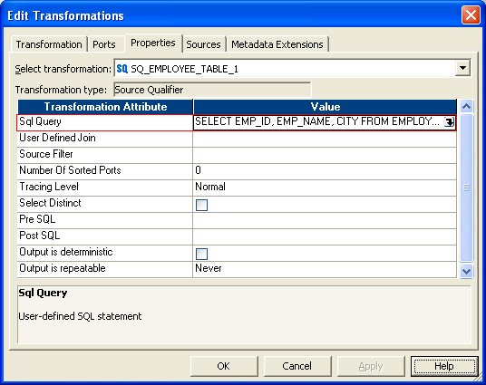
Add the above query to the source qualifier transformation in the Sql Query attribute value as shown below. This will override the default SQL query issued when the session runs. Ensure that the order of the columns in the SQL query match the order of the ports in the Source Qualifier.

The alias column 'SOURCE_NAME' value also needs to be passed to the target. For this purpose, a new port SOURCE_NAME is created in the source qualifier as shown below.

By default, all ports that are in the source qualifier are input/output ports. Hence, the new port SOURCE_NAME that is created should be linked to a field from the source definition having the same datatype i.e. the datatype varchar2 in the source definition changes to string in the source qualifier. If the port SOURCE_NAME is not linked, the session will fail with an error - TE_7020    Internal error. The Source Qualifier [SQ_EMPLOYEE_TABLE_1] contains an unbound field [SOURCE_NAME].

Link the CITY port from the source definition to the SOURCE_NAME port in the source qualifier. As a good practice, use an expression transformation in between the source qualifier and the target definition as shown below.

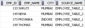
Create a session task and a workflow. After running the workflow, the difference rows loaded into the target relational table are shown below.

Understanding Oracle BI Applications

Oracle BI Applications are a complete, end-to-end BI environment covering the Oracle BI EE platform and the prepackaged analytic applications. The Oracle BI Applications discussed below is solely pertaining to its use with Informatica PowerCenter as the ETL tool. The current version of Oracle BI Applications which is intended for use with Informatica PowerCenter 8.6.1 is 7.9.6.1.

                                                           Courtesy: Oracle Corporation

As shown above, the packaged ETL mappings consume operational data from sources comprising J D

Edwards, Oracle, PeopleSoft and Siebel with the aid of source-specific adaptors as well as universal adaptors, which are used for legacy or other data sources. The data is then loaded into a data warehouse comprising of pre-built schemas, based on different subject areas, readily available for use with a reporting tool.

The main constituents of the Oracle BI Applications setup are the Informatica PowerCenter pre-packaged repository 'Oracle_BI_DW_Base.rep' that contains the pre-packaged ETL's, the metadata for the pre-built data warehouse referred to as the Oracle Business Analytics Warehouse (OBAW), the pre-built Oracle BI repository 'OracleBIAnalyticsApps.rpd' file that contains the pre-designed data models for different subject areas and the ready-to-use OBIEE web catalog 'EnterpriseBusinessAnalytics' that consists of pre-built dashboards and requests. The Oracle BI Applications provides a complete solution for enterprises needing a data warehouse having either one or more of the following source applications - J D Edwards, Oracle EBS, PeopleSoft and Siebel. The other installables needed for use with Oracle BI Applications includes Oracle Business Intelligence Enterprise Edition (OBIEE), Informatica PowerCenter and Data warehouse Administration Console (DAC).

Oracle BI Applications supplies the Informatica PowerCenter Standard Edition license in the Oracle_All_OS_Prod.key file. This license is non-expiry and supports a variety of platforms and databases and also offers PowerExchange licenses to access PeopleSoft, Oracle E-Business Suite, Siebel et al. The Informatica Administration Console is shown below that showcases the license information for different platforms, databases, source applications etc.

Oracle BI Applications provides a pre-built Informatica repository Oracle_BI_DW_Base.rep consisting of shared folders that contain packaged ETL mappings that extract data from sources comprising J D Edwards, Oracle, PeopleSoft and Siebel and load the data into the pre-built warehouse referred to as the Oracle Business Analytics Warehouse (OBAW). The image below shows the global repository Oracle_BI_DW_Base.

In the image, the  SDE_PSFT_89_Adaptor consists of mappings that extract data from PeopleSoft 8.9 application tables and loads them to the staging tables in the OBAW. SDE is Source Dependent Extract as the mapping depends on the source application for extraction of data and the mapping names in the SDE folders are pre-fixed with 'SDE_' like 'SDE_PSFT_EmployeeDimension' as shown below.

 

The SILOS folder comprises of mappings that load data into the dimension, fact and aggregate tables in the OBAW from the staging tables. The mappings in the SILOS folder are pre-fixed with 'SIL_' and SIL is referred to as Source Independent Loading.

The OBAW is administered by the DataWarehouse Administration Console (DAC). DAC not only facilitates the creation of the pre-built OBAW schemas, scheduling and monitoring the Informatica ETL process but also allows creation of customised tables, indices in the OBAW and also registering custom ETL tasks that are created in Informatica. DAC is an ETL orchestration tool that is used by warehouse developers and ETL administrators for application configuration, execution and recovery and monitoring. The DataWarehouse Administration Console is shown below.

Oracle also offers Oracle Data Integrator (ODI) as the middleware ETL tool as part of the Oracle BI Applications package, but it still continues to provide Informatica as the ETL solution as per the user's choice of middleware.

Oracle BI Applications provide a pre-built Oracle BI repository that comprises of different warehouse data models for a host of different applications that include Human Resources, Sales, Financials, Supply Chain and Order Management, etc. The contents of the Oracle BI repository file 'OracleBIAnalyticsApps.rpd' is shown below.

 

The image below shows the pre-built logical model for CRM - Revenue Fact comprising of one logical fact and several dimension tables. The ready-to-use model forms the basis for physical queries to be executed on the OBAW, when processing requests from Oracle BI Answers and Dashboards.

The pre-designed Oracle BI web catalog contains ready-to-use dashboards and requests, pertaining to different applications or subject areas. The image below shows the pre-built dashboard for Sales - Customers subject area's Account Summary page.

Thus, the Oracle BI Applications package is a complete, ready-to-use solution. However, the Oracle BI Applications implementation will either be a smooth ride if all the existing business logic is as per desired with minimal customizations or it may come with its own set of perils if there are data issues and major customizations in either the packaged ETL's or the pre-built OBIEE repository, requests or dashboards. But then everything that is readily delivered comes with its own set of pros and cons.