Reporting the difference rows between two sources using Informatica

The purpose of the mappings discussed below are to report the difference rows between two sources in different scenarios.

Scenario 1: When there are difference rows in one of the sources and both the sources are either flat files or a flat file and a relational table.
To illustrate this scenario, the two sources considered are two comma separated flat files - EMPLOYEE_FILE_1.txt and EMPLOYEE_FILE_2.txt. The EMPLOYEE_FILE_2.txt has some extra records that need to be reported or loaded into the target which is a relational table having the same definition as the sources. The difference rows between the two flat files are highlighted in red as shown below.

Import the two flat file definitions using the Source Analyzer in Informatica PowerCenter Designer client tool as shown below.

Create a new mapping in the Mapping Designer and drag the two source definitions into the workspace.
Now, to identify the extra records from EMPLOYEE_FILE_2, a Joiner transformation followed by a Filter transformation is used.

The illustration discussed below uses an unsorted Joiner Transformation and since both the sources are having few records, any one of the sources can be treated as the "Master" source. Here the EMPLOYEE_FILE_1 source is designated as the "Master" source. In practice, however, to improve performance for an unsorted joiner transformation, the source with fewer rows is treated as the "Master" source while for a sorted joiner transformation, the source with fewer duplicate key values is assigned as the "Master" source.

First drag all the ports from the source qualifier SQ_EMPLOYEE_FILE_2 into the joiner transformation. Notice the ports created in the joiner transformation are designated as the "Detail" source by default. Drag only the EMP_ID port from SQ_EMPLOYEE_FILE_1 into the joiner transformation as shown below.

Double-click the joiner transformation to open up the Edit view of the transformation. Click on the Condition tab and specify the condition shown below.

Since, we need to pass all the rows from the EMPLOYEE_FILE_2, the Join Type used is "Master Outer Join" in the Properties tab as shown below. This will ensure that all the rows from the "Detail" source and only the matching rows from the "Master" source will pass from the joiner transformation.

The Join types supported in the joiner transformation are described below.

The rows passed by the joiner transformation are shown below. For the missing rows in the "Master" source, the EMP_ID1 value is NULL.

Now, a filter transformation can be used ahead to pass only the records having EMP_ID1 as NULL since these rows correspond to the difference rows from EMPLOYEE_FILE_2 source. Pass all the rows from the joiner transformation into the filter transformation and add the Filter condition shown below in the Properties tab of the filter transformation.

The records passed by the filter transformation are shown below.

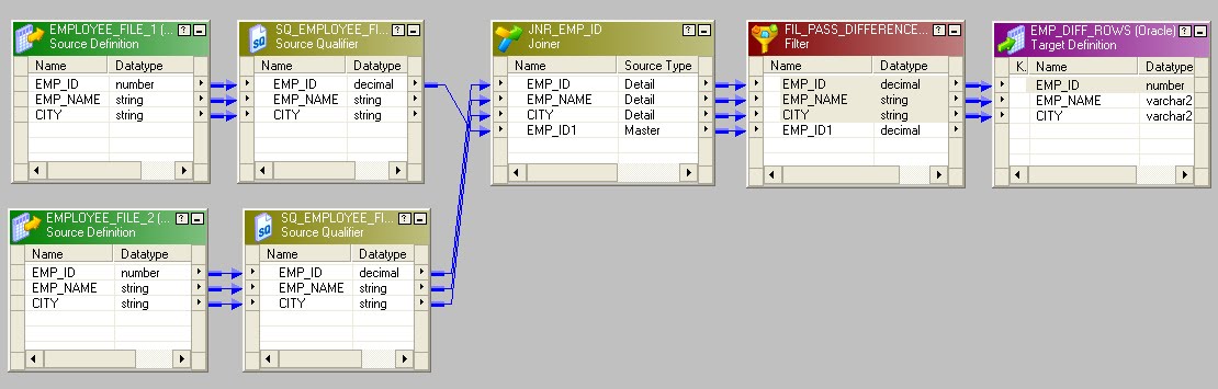
Link the EMP_ID, EMP_NAME and CITY ports to the target definition. The complete mapping is shown below.

Create a session task and a workflow. After running the workflow, the difference rows loaded into the target relational table are shown below.

Scenario 2: When there are difference rows in both the sources and both the sources are either flat files or a flat file and a relational table.
For this illustration, we consider both the sources are flat files. The difference rows in both the flat files are highlighted in red. The target relational table has an additional column SOURCE_NAME added, which indicates the source name where the difference row is present.

The EMPLOYEE_FILE_1 is treated as the "Master" source again for the unsorted joiner transformation. All the ports from the source qualifier SQ_EMPLOYEE_FILE_1 are passed to the joiner transformation as shown below because the difference records are present in both the sources.

The join condition for the joiner transformation is the same as the first scenario, but for this case, the Join Type is Full Outer Join as shown below.

The rows passed by the joiner transformation are shown below. For the missing rows in the "Master" source, the EMP_ID1, EMP_NAME1 and CITY1 values are NULL, while for the missing rows in the "Detail" source, the EMP_ID, EMP_NAME and CITY values are NULL.

The filter transformation shown below should only pass the rows having NULL values in EMP_ID or EMP_ID1 ports as these correspond to the difference rows in the EMPLOYEE_FILE_2 and EMPLOYEE_FILE_1 flat files respectively.

The filter condition used in the filter transformation is shown below.

The filter transformation passes the following rows.

Now, add an expression transformation after the filter transformation. Pass all the ports from the filter transformation to the expression transformation. The expression transformation should have the following ports in the order shown below.

The logic for the output port EMP_ID_OUT is that if the EMP_ID value from EMPLOYEE_FILE_2 source is NULL, pass the EMP_ID1 value from the EMPLOYEE_FILE_1 source, else return the EMP_ID value from EMPLOYEE_FILE_2 source. This logic works because for any row passed from the filter transformation, either the row from the "Master" source will have NULL values or the row from the "Detail" source will have NULL values. A similar logic is applied for the EMP_NAME_OUT and CITY_OUT output ports.

Another output port SOURCE_NAME_OUT is used to determine the source of the difference row. The expression used for this port is shown below.

The complete mapping is shown below.

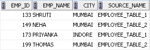
Create a session task and a workflow. After running the workflow, the difference rows loaded into the target relational table are shown below.

Scenario 3: When there are difference rows in two relational tables residing in the same database.
For this illustration, two relational tables EMPLOYEE_TABLE_1 and EMPLOYEE_TABLE_2 having the same definition are considered. The rows present in both the tables are shown below and the difference rows are highlighted in red.

Import the table definition of any one source in the Source Analyzer. Here, the EMPLOYEE_TABLE_1 source definition is imported.

A simple SQL query that returns the difference rows in EMPLOYEE_TABLE_1 is given below.

SELECT EMP_ID, EMP_NAME, CITY FROM EMPLOYEE_TABLE_1 EMP_1
WHERE NOT EXISTS (SELECT EMP_ID FROM EMPLOYEE_TABLE_2 EMP_2
WHERE EMP_1.EMP_ID = EMP_2.EMP_ID) 

The above query can be modified to return the difference rows between the two source tables and also the table name where the difference row is present. The alias column 'SOURCE_NAME' gives the source table name of the difference row.
SELECT EMP_ID, EMP_NAME, CITY, 'EMPLOYEE_TABLE_1' AS SOURCE_NAME
FROM EMPLOYEE_TABLE_1 EMP_1
WHERE NOT EXISTS (SELECT EMP_ID FROM EMPLOYEE_TABLE_2 EMP_2
WHERE EMP_1.EMP_ID = EMP_2.EMP_ID)
UNION
SELECT EMP_ID, EMP_NAME, CITY, 'EMPLOYEE_TABLE_2' AS SOURCE_NAME
FROM EMPLOYEE_TABLE_2 EMP_2
WHERE NOT EXISTS (SELECT EMP_ID FROM EMPLOYEE_TABLE_1 EMP_1
WHERE EMP_1.EMP_ID = EMP_2.EMP_ID)

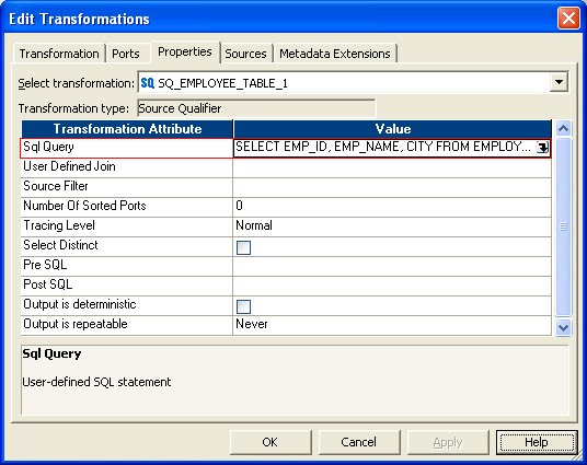
Add the above query to the source qualifier transformation in the Sql Query attribute value as shown below. This will override the default SQL query issued when the session runs. Ensure that the order of the columns in the SQL query match the order of the ports in the Source Qualifier.

The alias column 'SOURCE_NAME' value also needs to be passed to the target. For this purpose, a new port SOURCE_NAME is created in the source qualifier as shown below.

By default, all ports that are in the source qualifier are input/output ports. Hence, the new port SOURCE_NAME that is created should be linked to a field from the source definition having the same datatype i.e. the datatype varchar2 in the source definition changes to string in the source qualifier. If the port SOURCE_NAME is not linked, the session will fail with an error - TE_7020    Internal error. The Source Qualifier [SQ_EMPLOYEE_TABLE_1] contains an unbound field [SOURCE_NAME].

Link the CITY port from the source definition to the SOURCE_NAME port in the source qualifier. As a good practice, use an expression transformation in between the source qualifier and the target definition as shown below.

Create a session task and a workflow. After running the workflow, the difference rows loaded into the target relational table are shown below.

Understanding Oracle BI Applications

Oracle BI Applications are a complete, end-to-end BI environment covering the Oracle BI EE platform and the prepackaged analytic applications. The Oracle BI Applications discussed below is solely pertaining to its use with Informatica PowerCenter as the ETL tool. The current version of Oracle BI Applications which is intended for use with Informatica PowerCenter 8.6.1 is 7.9.6.1.

                                                           Courtesy: Oracle Corporation

As shown above, the packaged ETL mappings consume operational data from sources comprising J D

Edwards, Oracle, PeopleSoft and Siebel with the aid of source-specific adaptors as well as universal adaptors, which are used for legacy or other data sources. The data is then loaded into a data warehouse comprising of pre-built schemas, based on different subject areas, readily available for use with a reporting tool.

The main constituents of the Oracle BI Applications setup are the Informatica PowerCenter pre-packaged repository 'Oracle_BI_DW_Base.rep' that contains the pre-packaged ETL's, the metadata for the pre-built data warehouse referred to as the Oracle Business Analytics Warehouse (OBAW), the pre-built Oracle BI repository 'OracleBIAnalyticsApps.rpd' file that contains the pre-designed data models for different subject areas and the ready-to-use OBIEE web catalog 'EnterpriseBusinessAnalytics' that consists of pre-built dashboards and requests. The Oracle BI Applications provides a complete solution for enterprises needing a data warehouse having either one or more of the following source applications - J D Edwards, Oracle EBS, PeopleSoft and Siebel. The other installables needed for use with Oracle BI Applications includes Oracle Business Intelligence Enterprise Edition (OBIEE), Informatica PowerCenter and Data warehouse Administration Console (DAC).

Oracle BI Applications supplies the Informatica PowerCenter Standard Edition license in the Oracle_All_OS_Prod.key file. This license is non-expiry and supports a variety of platforms and databases and also offers PowerExchange licenses to access PeopleSoft, Oracle E-Business Suite, Siebel et al. The Informatica Administration Console is shown below that showcases the license information for different platforms, databases, source applications etc.

Oracle BI Applications provides a pre-built Informatica repository Oracle_BI_DW_Base.rep consisting of shared folders that contain packaged ETL mappings that extract data from sources comprising J D Edwards, Oracle, PeopleSoft and Siebel and load the data into the pre-built warehouse referred to as the Oracle Business Analytics Warehouse (OBAW). The image below shows the global repository Oracle_BI_DW_Base.

In the image, the  SDE_PSFT_89_Adaptor consists of mappings that extract data from PeopleSoft 8.9 application tables and loads them to the staging tables in the OBAW. SDE is Source Dependent Extract as the mapping depends on the source application for extraction of data and the mapping names in the SDE folders are pre-fixed with 'SDE_' like 'SDE_PSFT_EmployeeDimension' as shown below.

 

The SILOS folder comprises of mappings that load data into the dimension, fact and aggregate tables in the OBAW from the staging tables. The mappings in the SILOS folder are pre-fixed with 'SIL_' and SIL is referred to as Source Independent Loading.

The OBAW is administered by the DataWarehouse Administration Console (DAC). DAC not only facilitates the creation of the pre-built OBAW schemas, scheduling and monitoring the Informatica ETL process but also allows creation of customised tables, indices in the OBAW and also registering custom ETL tasks that are created in Informatica. DAC is an ETL orchestration tool that is used by warehouse developers and ETL administrators for application configuration, execution and recovery and monitoring. The DataWarehouse Administration Console is shown below.

Oracle also offers Oracle Data Integrator (ODI) as the middleware ETL tool as part of the Oracle BI Applications package, but it still continues to provide Informatica as the ETL solution as per the user's choice of middleware.

Oracle BI Applications provide a pre-built Oracle BI repository that comprises of different warehouse data models for a host of different applications that include Human Resources, Sales, Financials, Supply Chain and Order Management, etc. The contents of the Oracle BI repository file 'OracleBIAnalyticsApps.rpd' is shown below.

 

The image below shows the pre-built logical model for CRM - Revenue Fact comprising of one logical fact and several dimension tables. The ready-to-use model forms the basis for physical queries to be executed on the OBAW, when processing requests from Oracle BI Answers and Dashboards.

The pre-designed Oracle BI web catalog contains ready-to-use dashboards and requests, pertaining to different applications or subject areas. The image below shows the pre-built dashboard for Sales - Customers subject area's Account Summary page.

Thus, the Oracle BI Applications package is a complete, ready-to-use solution. However, the Oracle BI Applications implementation will either be a smooth ride if all the existing business logic is as per desired with minimal customizations or it may come with its own set of perils if there are data issues and major customizations in either the packaged ETL's or the pre-built OBIEE repository, requests or dashboards. But then everything that is readily delivered comes with its own set of pros and cons.

Feature Manipulation Engine (FME) and Informatica PowerCenter

Feature Manipulation Engine (FME) is a spatial ETL tool by Safe Software Inc.

The advantage of a spatial ETL tool is that it can read, write and even manipulate spatial data. While an ETL tool must have processing capabilities for the various column types that are in a non-spatial database or system, a spatial ETL must also have the spatial operations - geoprocessing capabilities that change the structure and representation of spatial data - needed to move from one spatial database or GIS to another.

Besides, FME can read data from and write data to over 250 supported formats. Informatica PowerCenter as an ETL tool cannot read from or write data in the spatial domain. So, the FME Extension for Informatica extends Informatica PowerCenter with spatial data integration capabilities.

You can read more on FME at http://www.safe.com/. Also, Safe Software Inc. provides a Free FME Evaluation Download that has 14 day free evaluation period. It also has a series of tutorials on how to get started with FME, how to register the FME Extension in an Informatica PowerCenter Repository Service as a plug-in and how to use the FME Extension for Informatica.

As shown below, the Oracle_BI_DW_Base Informatica Repository Service has registered the FME Client plug-in in the Administration Console.

Now, if we check the Informatica PowerCenter Designer client tool, we have a new transformation added i.e. the FME Transformation as shown below.

The FME transformation, if used within any Informatica PowerCenter mapping will enable spatial data flow within Informatica. FME is certainly a tool to explore, particularly if you are well-versed with the spatial domain.

Concatenating multiple fields from the source table as comma separated values into a field in the target table

The purpose of the mapping discussed below is to concatenate the employee skills data available in the EMPLOYEE_SKILLS source table and load it into the EMPLOYEE_SKILL_SUMMARY target table.

Below is the script for EMPLOYEE_SKILLS source table:

CREATE TABLE EMPLOYEE_SKILLS

(EMP_ID NUMBER(10),

EMP_NAME VARCHAR2(30),

EMP_SKILL1 VARCHAR2(40),

EMP_SKILL2 VARCHAR2(40),

EMP_SKILL3 VARCHAR2(40));

The data available in the EMPLOYEE_SKILLS table is shown below:

Below is the script for EMPLOYEE_SKILL_SUMMARY target table:

CREATE TABLE EMPLOYEE_SKILL_SUMMARY

(EMP_ID NUMBER(10),

EMP_NAME VARCHAR2(30),

EMP_SKILLS VARCHAR2(120));

The data from EMP_SKILL1, EMP_SKILL2 and EMP_SKILL3 columns of EMPLOYEE_SKILLS table should be concatenated as comma separated values into the EMP_SKILLS column of the EMPLOYEE_SKILL_SUMMARY table.

The mapping shown above is the earlier mapping which concatenated all the skill Input port values in the EMP_SKILL_OUT Output port in the EXP_CONCAT_SKILLS Expression Transformation. The expression used in the EMP_SKILL_OUT port is shown below.

The issue surfaced after the data was loaded in the target table. Below are the records loaded into the EMPLOYEE_SKILL_SUMMARY table.

Now, the EMP_SKILLS field was displayed in some analytical reports and the way the data showed up didn’t look very pleasing. For instance, EMP_ID = 1199 has no skills in the EMPLOYEE_SKILLS source table, so when the three input port values were concatenated in the expression transformation, the data displayed in the reports was ',,'. So, a logic needed to be implemented that took care of NULL values and didn’t add a ‘comma’ for the NULL values.

The new logic is discussed below.

Instead of concatenating all the EMP_SKILL1_IN, EMP_SKILL2_IN and EMP_SKILL3_IN port values together, the new logic checked if the Input Skill values in the ports EMP_SKILL1_IN and EMPSKILL2_IN were having NULL values. If it is a NULL value, it will pass a blank string as '', else it would concatenate the incoming value with a ‘comma’ in the variable ports EMP_SKILL1_V and EMP_SKILL2_V.

The EMP_SKILLS_CONCAT_V variable port will concatenate values from the variable ports EMP_SKILL1_V, EMP_SKILL2_V and the input port EMP_SKILLS3_IN.

Now, the only problem of a ‘comma’ occurring at the end of the concatenated string will be in a scenario when EMP_SKILL2_IN and EMP_SKILL3_IN values are NULL or when EMP_SKILL3_IN values is NULL. For instance, if we observe in the source table EMPLOYEE_SKILLS, for EMP_ID = 1127, the EMP_SKILL1 and EMP_SKILL2 columns have valid data. So, for this particular record, the EMP_SKILLS_CONCAT_V port will have the string value as ‘SQL Server 2005,OBIEE 10.1.3.4,’. At the end of the string, the extra comma gets added as well.

To eliminate this ‘comma’, the string in the variable port EMP_SKILLS_CONCAT_V is reversed in the variable port EMP_SKILLS_REVERSE_V. The EMP_SKILLS_REMOVE_COMMA_V variable port will check for the occurrence of a ‘comma’ at the start of the data string. If it encounters a comma, it will pass only the substring without the ‘comma’ at the start of the string, else it passes the data as it is. This is achieved with the expression as shown below.

Now, to get back the original concatenated string without any extra ‘comma’ , reverse the data again and pass it through the EMP_SKILLS_OUT output port to the final target table column EMP_SKILLS.

These are the records in the EMPLOYEE_SKILL_SUMMARY table after running the modified mapping again.